Rutile

Simple Rietveld refinement of Laboratory X-ray data of Rutile

TiO2 data were recorded on the durham d5000 with fixed slits and it is appropriate to refine a height correction. As you have a cif file for the material it can be read in directly. In cases where you don’t have a .cif file you’d click through the items in the “Structure – no cif” folder. If you’d like to see the structure in 3D click on “view_structure”. Then save the file and run it in TA.

Perform the following steps:

Start jEdit.

Click on the toolbar icon  . Select from the browser the file TA-Tutorials\data\rutile\d5_05005.raw. After selecting the data file an input file for running topas with the same name but extension .inp is created in the same directory.

The jEdit screen should now look something like the following:

The jEdit screen should now look something like the following:

Now we need to insert some keywords into the INP flie corresponding to things like anode used, instrument details and structural details.

Open the XInsert node called “TOPAS_Durham” then open the node called “Simple Lab Rietveld”. The jEdit screen should look like the following:

Click on node called “File Header”. This inserts some default keywords like r_wp etc…

The jEdit screen should now look like the following:

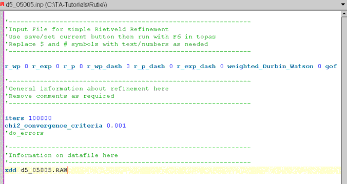
Position the cursor on the line with the xdd keyword.

Click on node called “Background”. This inserts the keyword bkg which defines the coefficents of a Chubychev polynomial.

The jEdit screen should now look like the following:

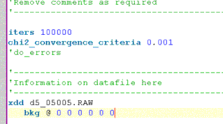
Thus using jEdit to create INP file involves working ones way down the XInsret treeview and inserting items as required.

Perform the following to complete the setting up of the Rutile INP file.

Open the XInsert node “Instrument/Corrections” and click on “Durham_d5000”.

Click on “Refine zero point”.

Click on “Refine sample height”. N.B. zero point and height are highly correlated so you would normally refine one or the other.

Open the “Structure – cif” node and click on “Read a CIF file”. Browse to TA-Tutorials\data\rutile\rutile.cif and select it. The jEdit screen should now look like the following:

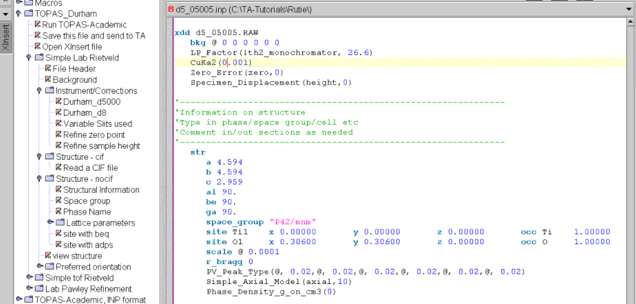
Now we are ready to do a preliminary refinement on the data set.

Click on the icon  to start TA. Note, once TA is started it is not necessary to start it again.

Click on the icon  which sends the name of the present INP file to a text file in the main TA directory called LAUNCH_FILE.TXT. This simply instructs TA to operate on this INP file.

Alt-Tab to TA and press the Fit Window icon ; this starts the refinement.

After refinement the TA screen should look like the following:

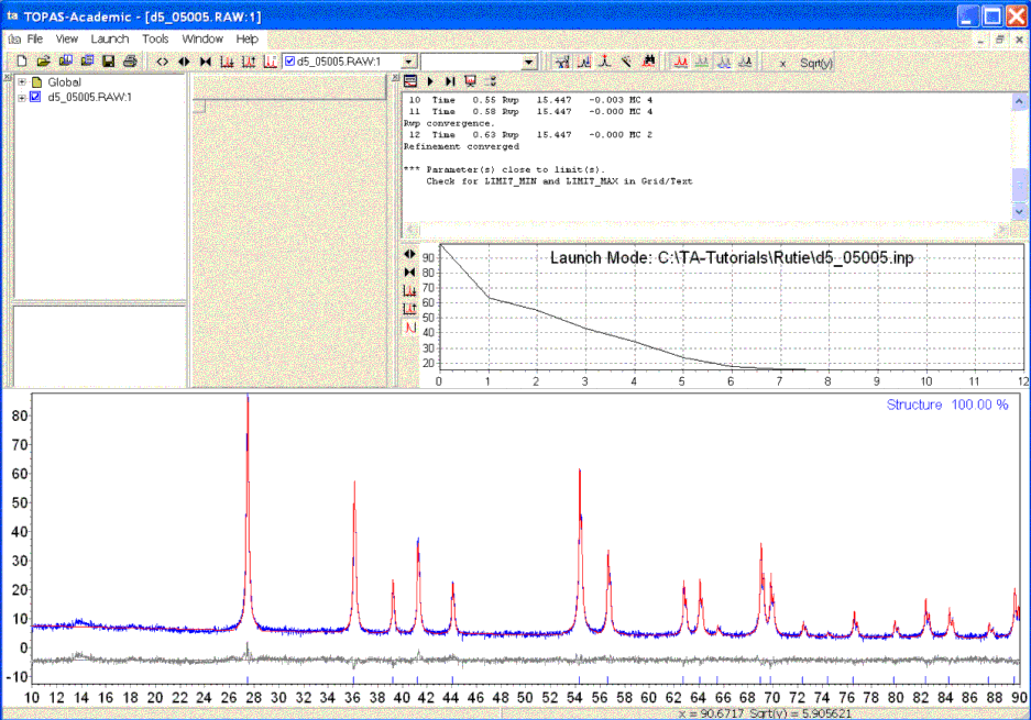
TA automatically loaded the observed pattern (blue) and then shows the calculated pattern in red after each refinement iteration.

Alt-Tab back to jEdit. jEdit will automatically load the modifed INP file with refined parameter values updated and in red. The jEdit screen should look like the following:

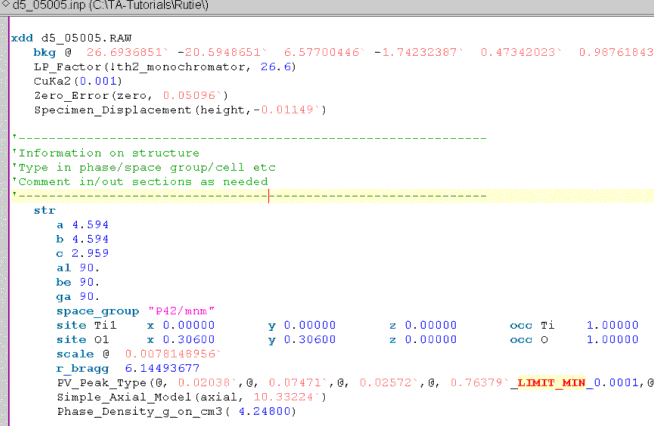
This CIF file did not include any temperature factors (typically they do); thus add them manually by appending to the end of each site line “beq @ 1”.

Save the INP file by pressing Alt-w (if INP keystrokes are implemented) or File/Save or click on the icon .

Alt-Tab back to TA and run the refinement again; the Rwp should drop by around 0.9% with the beq values refining.

Place the jEdit cursor somewhere after the “str” keyword and click on “view_structure”. Save and run the refinement again. Now you should see the structure displayed in an OpenGL window.

To instruct TA to calculate errors for the refined parameters; uncomment out the “do_errors” line at the top of the INP file; ie. remove the line comment character of ‘.

Save the INP file by pressing Alt-w or click on the icon .

Alt-Tab to TA and run the refinement.

Alt-Tab to jEdit and the INP file should now look like the following:

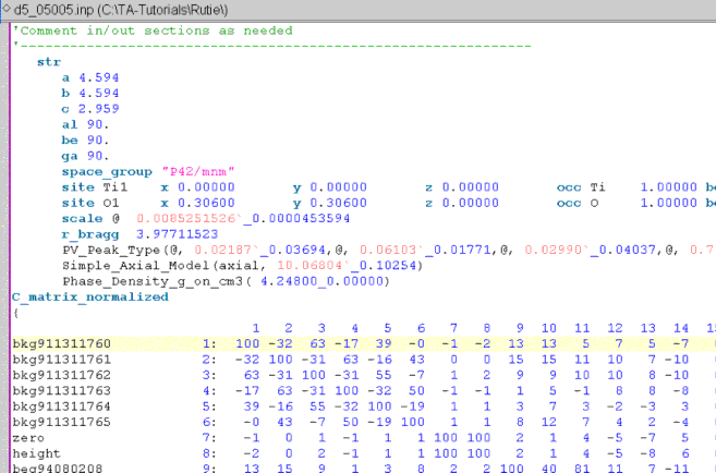
Appended to refined parameter values (red numbers) is an underscore followed by a number; these numbers are the errors.

Also, the keyword C_matrix_normalized is appended to the bottom of the INP file (if it does not already exist). Following the C_matrix_normalized keyword is the normalized correlation matrix.

This completes the tutorial.